Understanding the Role of Photoelectric Sensors in PID Control
In industrial automation, photoelectric sensors are widely used for non-contact detection of objects, position, and distance. When integrating a PID (Proportional-Integral-Derivative) controller with a photoelectric sensor, the sensor provides real-time feedback on process variables such as light intensity, target position, or distance. This feedback is critical for closed-loop control systems that require precise regulation. For example, in conveyor belt systems or robotic arm alignment, the sensor’s analog output (e.g., 0-10V or 4-20mA) is fed into a PLC or microcontroller, which then calculates the PID output to adjust actuators like motors or valves. A well-structured PID program minimizes overshoot, reduces steady-state error, and ensures system stability under varying conditions.
Key Components of a PID Algorithm for Sensor Feedback
A PID program for a photoelectric sensor typically involves three main components: proportional (P), integral (I), and derivative (D) terms. The proportional term responds to the current error (difference between setpoint and measured value), the integral term accumulates past errors to eliminate steady-state offset, and the derivative term predicts future trends to dampen oscillations. For photoelectric sensors, the sampling rate must be high enough to capture rapid changes in the sensed signal—typically 10-100 Hz depending on the application. Additionally, anti-windup mechanisms are essential for the integral term to prevent saturation when the sensor is blocked or the output is limited. Engineers should also consider sensor noise filtering, often via a low-pass filter, to avoid derivative kick.
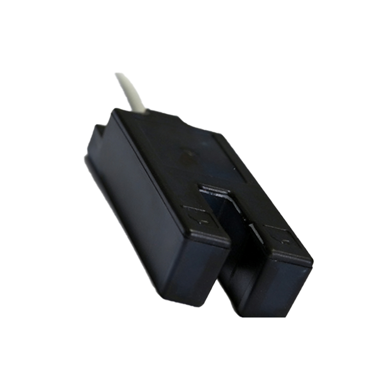
Step-by-Step PID Program Structure for PLC Integration
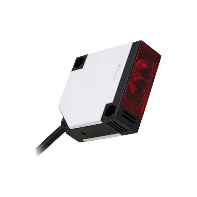
To write a PID program for a photoelectric sensor in a PLC environment (e.g., using ladder logic or structured text), follow these steps: 1. Initialize sensor input—assign an analog input channel to read the sensor voltage or current. 2. Set the target setpoint based on desired process conditions (e.g., 5V for a specific distance). 3. Calculate error = setpoint - process variable. 4. Compute P term = Kp * error. 5. Compute I term = Ki * integral of error over time (use a dedicated accumulator). 6. Compute D term = Kd * derivative of error (or process variable). 7. Sum all terms to get PID output, then clamp it within actuator limits (e.g., 0-100% PWM duty cycle). 8. Update integral accumulator with anti-windup logic (e.g., stop integrating if output is saturated). 9. Loop back at a fixed interval using a timer. In structured text, you can use functions likePID_EXE in many PLCs, but custom code gives more flexibility for sensor-specific tuning.
Tuning PID Parameters for Photoelectric Sensor Applications
Proper tuning is crucial for reliable operation with photoelectric sensors. Start with the Ziegler-Nichols method: set Ki and Kd to zero, increase Kp until the system oscillates (critical gain Kc), then calculate Kp=0.6*Kc, Ki=2*Kp/period, Kd=Kp*period/8. For photoelectric sensors, the derivative term is often set low or disabled if noise is present. In applications like object detection (binary signals), PID may be unnecessary—use on/off control instead. But for analog sensors measuring distance or light intensity, fine-tune by observing step response: reduce overshoot with D term, and eliminate offset with I term. Always test under worst-case conditions (e.g., dust, ambient light changes) to ensure robustness.
Practical Example: PID Program for a Distance-Measuring Photoelectric Sensor
Consider a scenario where a photoelectric sensor outputs 0-10V corresponding to 0-100mm distance, and the target is 50mm (5V). In a Siemens S7-1200 PLC using TIA Portal, you can implement a PID compact instruction. Configure the sensor input as an analog tag (e.g.,Sensor_Value). Set the setpoint to 50.0. In the PID block, set proportional gain to 2.0, integral time to 0.5 seconds, derivative time to 0.1 seconds, and sampling time to 0.01 seconds. The output controls a linear actuator via analog or PWM. During commissioning, monitor the response curve—if overshoot exceeds 10%, reduce Kp or increase Kd. If steady-state error persists, increase Ki slowly. For noisy signals, add a moving average filter in the program before the PID input. This approach ensures smooth and accurate positioning in automated assembly lines.
Common Challenges and Solutions in PID Implementation
Engineers face several challenges when programming PID for photoelectric sensors. First, sensor signal drift due to temperature or aging can cause offset—mitigate by adding automatic recalibration or using a derivative-only term. Second, response lag if the sensor has a slow update rate—choose sensors with fast response times (<1ms) for dynamic processes. Third, integral windup when the sensor is blocked—use conditional integration or clamp the integral term. Fourth, noise from electromagnetic interference—shield cables and apply digital filters. Finally, ensure the PID loop runs at a consistent frequency; avoid blocking operations like communication in the same scan cycle. Document all tuning parameters and test scenarios to simplify future maintenance.