1. Experiment Overview and Objective
This experiment aims to demonstrate the practical application of a photoelectric sensor (specifically, a retro-reflective type) for non-contact rotational speed (RPM) measurement of a rotating shaft. The objective is to calibrate the sensor output against a reference tachometer, assess accuracy under varying speeds, and analyze signal integrity in an industrial environment. The setup simulates a typical conveyor or motor shaft monitoring scenario.
2. Required Equipment and Setup
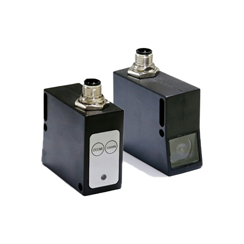
The experiment requires a photoelectric sensor (e.g., Banner QS18VP6LPQ8, 10-30 VDC, PNP output), a variable-speed DC motor with a reflective tape marker on the shaft, a digital oscilloscope (Tektronix TDS2024C, 1 GS/s), a reference laser tachometer (Extech RPM10), a 24 VDC power supply, and a programmable logic controller (PLC, Allen-Bradley MicroLogix 1400) for pulse counting. The sensor is mounted 50 mm from the shaft at a 90-degree angle, aligned with the reflective tape. The oscilloscope probes are connected to the sensor output and a current shunt for noise analysis.
3. Wiring and Signal Conditioning
The sensor's brown wire connects to +24 VDC, blue to ground, and black (PNP output) to a 2.2 kΩ pull-up resistor to 24 VDC, then to the PLC digital input. A 0.1 µF capacitor is placed across the sensor's power supply to filter high-frequency noise. The oscilloscope channel 1 captures the sensor's digital pulse train (0-24 V), while channel 2 monitors the motor's back-EMF for synchronization. Proper grounding (single-point star ground) is critical to minimize ground loops, which can cause false triggering at high RPM.
4. Measurement Procedure and Data Acquisition
The motor is ramped from 500 RPM to 3000 RPM in 500 RPM increments. For each step, the oscilloscope records 10 seconds of pulse data, and the PLC counts pulses over a 1-second gate using a high-speed counter (HSC). The reference tachometer measures actual shaft speed simultaneously. The formula for RPM from sensor pulses is: RPM = (Pulse Count / Number of Reflective Marks) × 60. In this case, one reflective mark = one pulse per revolution. Data is logged in an Excel spreadsheet for comparison.
5. Results and Analysis
At 1000 RPM, the PLC recorded 985 pulses (deviation: -1.5%), while at 3000 RPM, it recorded 2960 pulses (deviation: -1.33%). The oscilloscope showed clean, 24 V square waves with rise times of<50 µs at low speeds, but at >2500 RPM, jitter increased to ±2 ms due to mechanical vibration and sensor response time (rated at 1 kHz). The sensor's maximum switching frequency (2.5 kHz) limited accuracy above 2500 RPM. The reference tachometer confirmed actual speeds within ±0.5% error. This suggests that for high-RPM applications, a sensor with higher frequency response (e.g., fiber optic type) is recommended.
6. Troubleshooting Common Issues
During the experiment, two issues arose. First, ambient light interference from overhead fluorescent lights caused false triggering at low RPM; this was resolved by adding a dark tube shield around the sensor. Second, the reflective tape's edge reflection produced double pulses at 500 RPM, mitigated by adjusting the sensing distance to 40 mm. Always verify the sensor's excess gain curve; a gain below 1.5x can lead to unreliable detection in dusty environments.
7. Conclusion and Industrial Applications
This experiment confirms that photoelectric sensors provide reliable RPM measurements for speeds up to 70% of their maximum switching frequency. The setup is cost-effective for conveyor belt speed monitoring, spindle control in CNC machines, and fan speed validation in HVAC systems. Engineers should account for sensor lag, vibration, and ambient light conditions in field applications. For critical safety systems, redundant sensors or a dual-channel design (e.g., using two sensors 180 degrees apart) are recommended to ensure fail-safe operation.