Understanding the Basics of Numerical Photoelectric Sensors
Numerical photoelectric sensors are critical components in modern industrial automation, providing precise detection of objects, distances, and positions. These sensors operate by emitting a beam of light and measuring the reflected or interrupted signal to determine the presence or absence of a target. Unlike traditional binary sensors, numerical models offer analog outputs or digital interfaces (e.g., IO-Link), allowing for fine-tuned adjustments and data feedback. For effective adjustment, engineers must first understand the sensor’s operating principle, such as through-beam, retro-reflective, or diffuse modes, as each requires specific alignment and sensitivity settings. Always consult the manufacturer’s datasheet for voltage, current, and environmental limits before starting.
Pre-Installation Checks and Mounting Considerations
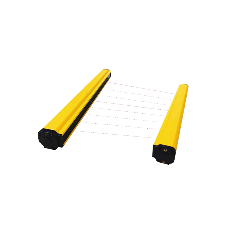
Before adjusting the sensor, ensure proper mounting and alignment. Use a stable bracket to avoid vibration-induced errors. For through-beam sensors, align the emitter and receiver coaxially, with no obstructions in the light path. For retro-reflective sensors, mount the reflector perpendicular to the beam. For diffuse sensors, consider the target’s surface reflectivity and color, as dark or matte objects may require higher sensitivity. Perform a visual check for dust, moisture, or ambient light interference, especially in harsh industrial environments. Secure all cables and connectors to prevent signal noise.
Initial Power-On and Parameter Configuration
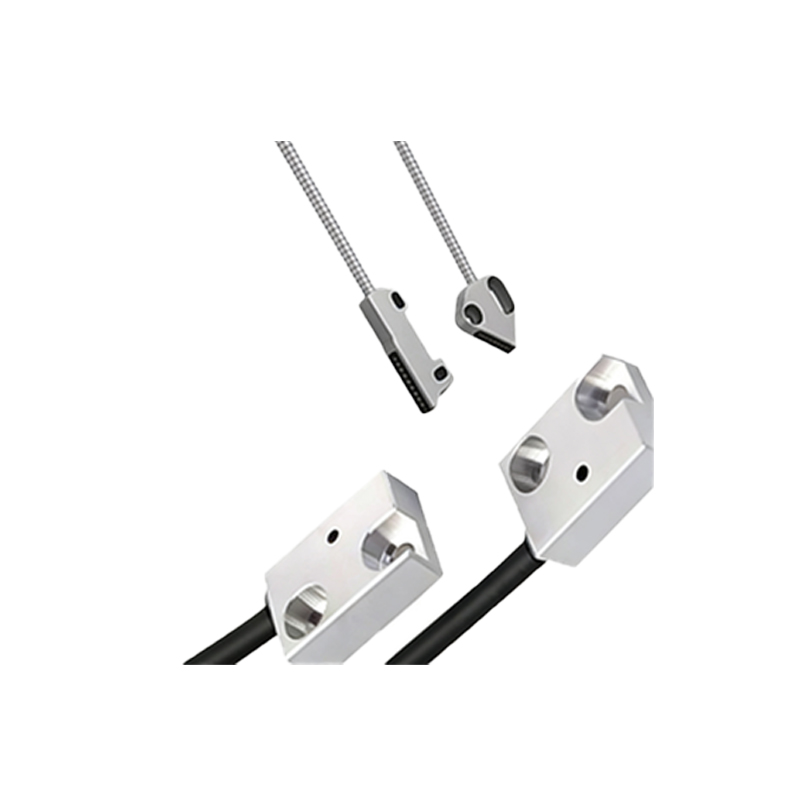
Connect the sensor to the control system (e.g., PLC) and power it on. Most numerical photoelectric sensors feature a teach-in button or software interface for parameter setup. Start by setting the operating mode (e.g., Light-ON or Dark-ON) based on your application. For example, in a conveyor belt system, use Light-ON to detect object presence when the beam is blocked. Access the sensor’s menu via a programming tool or IO-Link master to configure response time, hysteresis, and output logic. Use a multimeter or oscilloscope to verify signal integrity during initial tests.
Calibrating Sensitivity and Detection Distance
Adjust sensitivity using the sensor’s potentiometer or digital teach function. For diffuse sensors, place a standard target at the desired detection point (e.g., 100 mm) and press the teach button to auto-calibrate the threshold. For through-beam sensors, set sensitivity to maximum to ensure reliable detection over long distances. Use the sensor’s numerical display or software to monitor signal strength (e.g., 0-100% scale). A typical good signal is above 80% for robust detection. Avoid over-adjusting, as high sensitivity may cause false triggers from background objects or reflections.
Fine-Tuning with Real-Time Feedback
Simulate real operating conditions by running the target through the sensor’s detection zone while observing the output. Use a scope or the sensor’s internal logging to check for jitter, missed detections, or excessive triggering. Adjust the hysteresis (e.g., 5-10% of the signal range) to prevent oscillation near the threshold. For high-speed applications, reduce response time (e.g., 0.5 ms) but ensure the sensor’s switching frequency supports it. If using IO-Link, retrieve process data to optimize parameters like window comparator settings for precise object positioning.
Troubleshooting Common Issues
Common problems include false triggers, no output, or unstable signals. Check alignment first: even a 1-degree misalignment can reduce signal strength by 30%. Clean the lens and reflector with a lint-free cloth. For ambient light interference, use a modulation frequency filter or shield the sensor. If the sensor fails to detect transparent or glossy objects, switch to a polarizing filter or change the sensing mode. Update firmware if available. Document all changes in a maintenance log for future reference.
Final Validation and Integration into System
After adjustment, run a full production cycle to validate performance. Measure repeatability (e.g., ±0.1 mm) and response consistency. Integrate the sensor’s output into the PLC program, mapping analog values to engineering units (e.g., 4-20 mA = 0-500 mm). Perform a fallback test by simulating sensor failure to ensure the system enters a safe state. Record the final configuration parameters, such as sensitivity setting, threshold values, and IO-Link parameters, on the sensor’s label or in a database.