Introduction to Proximity Sensor Calibration
Proximity sensor calibration is a fundamental procedure in industrial automation and control systems. It ensures that the sensor's output accurately reflects the true distance to a target object within its specified sensing range. Without proper calibration, even a high-quality sensor can produce unreliable data, leading to process inefficiencies, quality control issues, or machine failures. The calibration process involves adjusting the sensor's internal parameters so that its electrical output signal—whether analog (e.g., 4-20 mA, 0-10 V) or digital—corresponds linearly and precisely to a set of known physical distances. This procedure is critical for applications requiring precise positioning, object detection, or thickness measurement, where millimeter or even micron-level accuracy is demanded.
Core Operating Principles Behind Calibration
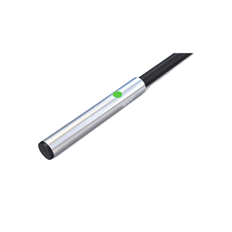
Understanding calibration requires a grasp of core sensing technologies. Inductive sensors generate an electromagnetic field and detect changes caused by conductive metallic targets. Capacitive sensors create an electrostatic field and react to any material that alters capacitance. Ultrasonic sensors measure the time-of-flight of sound waves, while photoelectric sensors use light beams. Each technology has a unique transfer function—the mathematical relationship between distance (input) and output signal. Calibration essentially defines and fine-tunes this function. For instance, in a typical analog inductive sensor, the calibration process maps the minimum sensing distance (Smin) to the minimum output (e.g., 4 mA) and the maximum sensing distance (Smax) to the maximum output (e.g., 20 mA), ensuring a linear response across the range.
Key Parameters and Calibration Points
Several key parameters are defined during calibration. The "calibrated sensing range" is the span between Smin and Smax where the sensor guarantees specified performance. "Linearity error" refers to the maximum deviation of the actual response curve from the ideal straight line, often expressed as a percentage of the full scale. "Hysteresis" is the difference in output when the target approaches the sensor versus when it recedes, measured at the same distance. Effective calibration minimizes these errors. Calibration is typically performed at multiple points—at least at zero (or Smin), span (Smax), and often a midpoint—to verify linearity. High-precision calibration may use five or more points across the range to create a more accurate correction curve or lookup table.
Step-by-Step Calibration Procedure
A standard calibration procedure follows a systematic approach. First, the sensor is mounted in a fixed, vibration-free fixture. A calibration target, made of the standard material specified for the sensor (e.g., mild steel for inductive), is attached to a high-precision linear positioning stage. The target is moved to the known Smin position, and the corresponding output signal is measured. The sensor's zero or offset potentiometer or digital parameter is adjusted until the output matches the desired low-scale value. Next, the target is moved to the Smax position, and the span or gain adjustment is made to achieve the correct high-scale output. This two-point adjustment is iterated until both points are accurate. Finally, the target is moved to several intermediate points to verify linearity; if errors exceed specifications, further digital linearization may be required.
Interpreting Calibration Diagrams and Curves
Calibration diagrams are essential tools for understanding sensor performance. The primary diagram is the "Distance vs. Output Characteristic Curve." This graph plots the physical distance on the X-axis against the electrical output (voltage, current, or digital value) on the Y-axis. The ideal calibration yields a perfectly straight line from (Smin, Output_min) to (Smax, Output_max). The actual calibrated curve is plotted alongside, and the shaded area between the two lines represents the linearity error. Another crucial diagram is the "Hysteresis Curve," which forms a loop showing the output path during approach and retreat. Diagrams also often include "Temperature Drift" curves, showing how the calibration shifts with ambient temperature changes, highlighting the need for temperature-stable environments or compensated sensors.
The Role of Digital Communication and Smart Sensors
Modern "smart" proximity sensors with IO-Link, PROFINET, or other digital interfaces have revolutionized calibration. These sensors store calibration data—including zero point, span, linearization coefficients, and even temperature compensation values—directly in their memory. Calibration can be performed via software, with results digitally logged. The sensor can often output its own health status, including warnings for calibration drift. Furthermore, digital sensors allow for "parameter switching," where different calibrated settings (e.g., for different target materials) can be stored and selected on command, providing immense flexibility. The calibration diagram for