In the realm of industrial automation, proximity sensors are indispensable for non-contact detection, and among them, metal-sensing variants are the most prevalent. A critical tool for engineers to select, apply, and troubleshoot these sensors is the characteristic curve, often found in the sensor's datasheet. This graphical representation is far more than a simple specification; it is a comprehensive performance map that dictates the sensor's behavior in real-world conditions.
The primary axis of a standard characteristic curve plots the sensing distance (Sn) against the target material. The most prominent feature is the rated operating distance (Sn). This value, typically defined for a standard target of mild steel (e.g., Fe360), represents the nominal switching distance under ideal conditions—23°C (±5°C) and a supply voltage at nominal rating. It is crucial to understand that Sn is not the maximum possible distance but a reliable, repeatable benchmark. The curve will clearly show that for different metals, the effective sensing distance varies significantly. For instance, a sensor calibrated for steel will exhibit a reduced sensing distance for non-ferrous metals like aluminum or copper. This reduction factor, often presented as a correction coefficient (e.g., 0.4 for aluminum), is directly readable from comparative plots on the curve. This is due to the differing effects of eddy currents and magnetic fields on various materials.
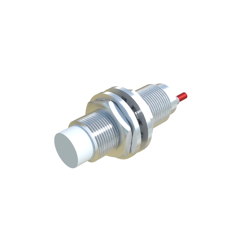
Another vital set of lines on the characteristic curve defines the limits of operation. The usable operating distance (Su) accounts for manufacturing tolerances and environmental factors like temperature and voltage fluctuations. It typically ranges from 90% to 110% of Sn. This zone ensures reliable switching despite variations. Beyond Su lies the assured operating distance (Sa), which represents the absolute limits within which switching is guaranteed, considering all permissible influences like temperature, voltage, and component aging. Installing a target within Sa guarantees functionality, while placement between Sa and Su might work but is not assured under all conditions. The curve also demarcates the non-sensing zone close to the sensor face and the hysteresis zone, which prevents chatter by creating a differential between the switch-on and switch-off points.
Temperature drift is a critical performance parameter graphically illustrated on these curves. Separate lines often show the shift in operating distance across the sensor's specified temperature range (e.g., -25°C to +70°C). A well-designed sensor will exhibit minimal drift, represented by nearly parallel lines close to the Sn line. A significant spread indicates higher temperature sensitivity, which could lead to unreliable detection in environments with wide thermal swings. Similarly, the influence of supply voltage on the sensing distance may be shown. A stable sensor will maintain a consistent Sn across its rated voltage range, a feature evident from a flat characteristic line in the voltage vs. distance plot.
For cylindrical sensors, the axis of approach is another factor depicted. The characteristic curve specifies whether the sensing distance is defined for an axial approach (target moving towards the face) or a radial approach (target moving past the side). The effective sensing distance can differ between these approaches, and the correct interpretation prevents mounting errors. Furthermore, the curve provides information on the repeatability of switching points, a key metric for precision applications. This is usually expressed as a percentage of Sn and indicates the sensor's consistency over millions of operating cycles.
In practical application, engineers use these curves to size sensors correctly, ensuring the target enters the reliable Sa zone. They aid in diagnosing issues—if a sensor intermittently fails, consulting the characteristic curve for temperature effects or material correction factors often reveals the root cause. For example, replacing a steel target with a stainless steel one, which has lower permeability, without consulting the correction factor will result in a failure that the curve would have predicted. Ultimately, mastering the interpretation of the metal proximity sensor characteristic curve transforms it from a datasheet graphic into a powerful engineering tool for optimizing system reliability, performance, and maintenance planning. It enables precise selection, prevents common installation pitfalls, and provides a scientific basis for troubleshooting, ensuring seamless integration within complex automated systems.