Understanding the Fundamentals of Photoelectric Sensors
Photoelectric sensors are critical components in industrial automation, converting light signals into electrical outputs for object detection, distance measurement, and process control. A typical programming diagram integrates sensor logic with programmable logic controllers (PLCs) or microcontrollers, using binary or analog signals. Engineers must first grasp the sensor types—through-beam, retro-reflective, and diffuse—each requiring distinct wiring and code configurations. For instance, a through-beam sensor uses a separate emitter and receiver, demanding precise alignment in the diagram, while retro-reflective models rely on a reflector and require less setup. Understanding these basics ensures accurate sensor integration, reducing false triggers and improving system reliability.
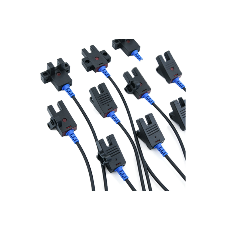
Decoding the Wiring and Pin Configuration
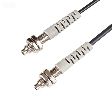
The programming diagram begins with a clear wiring schematic, often using color-coded pins: brown for power (24V DC), blue for ground, black for output (NPN or PNP), and white for test or auxiliary functions. For NPN outputs, the load connects between the output and positive supply, while PNP outputs connect between output and ground. Engineers must confirm the sensor’s datasheet to avoid short circuits. In the diagram, include a fuse or current-limiting resistor for protection. For example, a standard wiring setup for a diffuse sensor might show the black wire tied to a PLC input module, with a pull-up resistor for noise immunity. This clarity prevents installation errors and speeds up troubleshooting.
Configuring Sensor Parameters via Software
Modern photoelectric sensors offer programmable parameters through software tools like IO-Link or proprietary interfaces. The programming diagram should detail the communication protocol: typically, I²C or SPI for embedded systems, or discrete I/O for older models. Key parameters include sensitivity (threshold adjustment), response time (e.g., 1 ms to 10 ms), and output logic (normally open or normally closed). For instance, in a high-speed conveyor system, set the response time to 1 ms to detect fast-moving objects. The diagram must show the logic flow: if sensor output is high and timer expires, trigger a reject signal. Always document the default values to revert if needed.
Creating the Logic Flow for Object Detection
The core of a programming diagram is the logic flow, often represented as a state machine or ladder logic. Start with initialization: power-up sequence, sensor warm-up (typically 100 ms), and self-test (checking for internal faults). Then, the detection loop: read the sensor output, compare it against a predefined threshold, and execute an action—like activating a solenoid or sending an alert. For example, in a sorting system, the diagram might show a counter incrementing on each detection, with a diverter activating after 10 counts. Include hysteresis to avoid oscillation near the threshold, such as a 5% margin. This structured approach ensures robust performance in noisy environments.
Testing, Calibration, and Debugging Tips
After programming, testing is vital. The diagram should include calibration steps: use a standard target (e.g., a white card for diffuse sensors) to set the sensitivity, then verify with actual objects. For debugging, include a test mode in the software that outputs raw signal values to a diagnostic tool. Common issues include crosstalk between multiple sensors—mitigate by mounting them at angles or using different frequencies. In the diagram, add a status LED indicator (e.g., green for good, red for error) to quickly identify faults. Document these steps to streamline field maintenance and reduce downtime.