For electrical engineers and automation professionals, proximity sensors are indispensable components in modern industrial systems. Their ability to detect the presence or absence of an object without physical contact makes them vital for applications ranging from assembly lines to safety systems. However, to ensure optimal performance and reliability, one must thoroughly understand how to interpret their sensing curves. This guide provides a detailed walkthrough of reading and analyzing these critical graphs.
A sensing curve, often referred to as a sensing characteristic curve or response curve, graphically represents the relationship between the sensing distance and various influencing factors. Typically, the horizontal axis (X-axis) denotes the distance from the sensor face to the target object, while the vertical axis (Y-axis) indicates the sensor's output signal or sensitivity. The most common type is the "sensing distance vs. target material/size" curve, which shows how detection range varies with different target materials, such as steel, aluminum, copper, or non-metallic substances. For inductive proximity sensors, ferrous metals like steel yield the longest sensing distances, while non-ferrous metals reduce the effective range. Capacitive sensors, on the other hand, respond to a wider variety of materials but may require calibration based on dielectric constants.
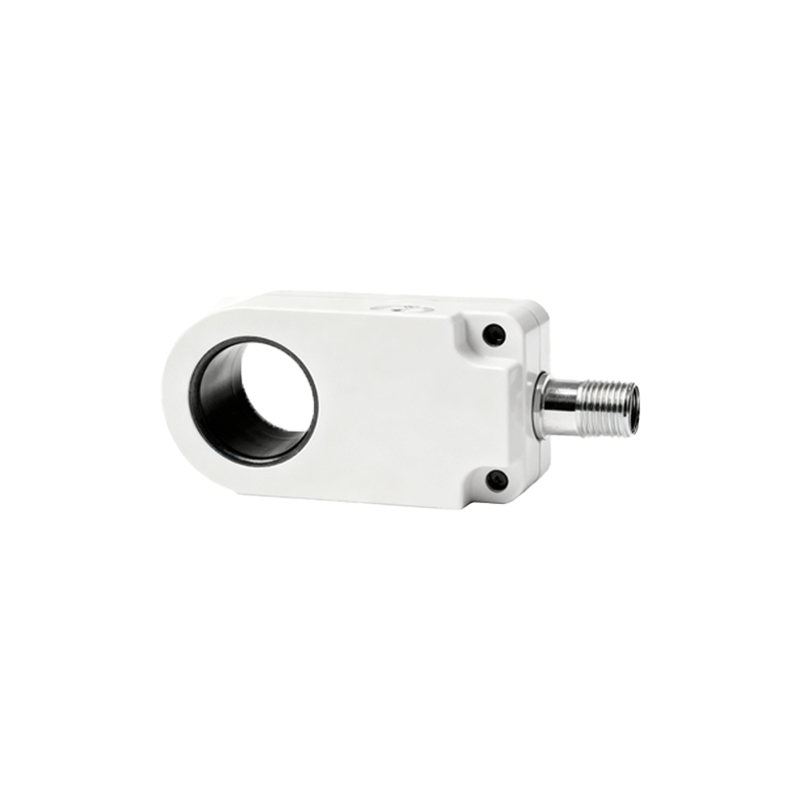
When examining a sensing curve, start by identifying the rated sensing distance (Sn). This is the nominal detection range specified under standard conditions, usually with a standard target (e.g., a square steel plate of defined dimensions). The curve often plots the actual sensing distance as a percentage of Sn. For instance, if a sensor has an Sn of 10 mm, the curve might show that for aluminum, the sensing distance drops to 60% of Sn, or 6 mm. This highlights the importance of material correction factors. Additionally, pay attention to the hysteresis zone—the difference between the switch-on point (when the sensor detects the approaching target) and the switch-off point (when the target moves away). Hysteresis prevents output oscillation near the detection threshold and is typically depicted as a gap between two lines on the curve. A larger hysteresis enhances stability but may reduce precision in positioning applications.
Environmental factors also play a crucial role in sensing curves. Temperature variations can shift the curve, as most sensors experience thermal drift. Manufacturers often provide separate curves for different temperature ranges, showing how sensing distance changes with ambient heat or cold. For example, at high temperatures, the effective range might decrease due to changes in coil resistance or electronic components. Similarly, voltage fluctuations can affect output, so curves may include lines for minimum and maximum supply voltages. Always cross-reference these with your operating conditions to avoid false triggers or missed detections.
Another key aspect is the target size and orientation. Sensing curves are typically derived using standard targets, but real-world objects may be smaller or shaped differently. Many curves include auxiliary graphs showing reduction factors for smaller targets. If a target is less than the sensor's face diameter, the sensing distance decreases proportionally. Orientation matters too: a flat surface perpendicular to the sensor axis provides maximum range, while angled surfaces reduce it. Some advanced curves incorporate 3D diagrams to illustrate these effects, helping engineers design layouts that account for target alignment.
Interpreting dynamic response curves is essential for high-speed applications. These curves plot response time versus sensing distance, indicating how quickly the sensor can detect a moving target. Factors like target speed, sensor switching frequency, and output delay (e.g., for analog or digital signals) are depicted. For instance, a curve might show that at full sensing distance, response time increases slightly due to signal processing. Understanding this prevents errors in timing-critical tasks, such as counting fast-moving items on a conveyor.
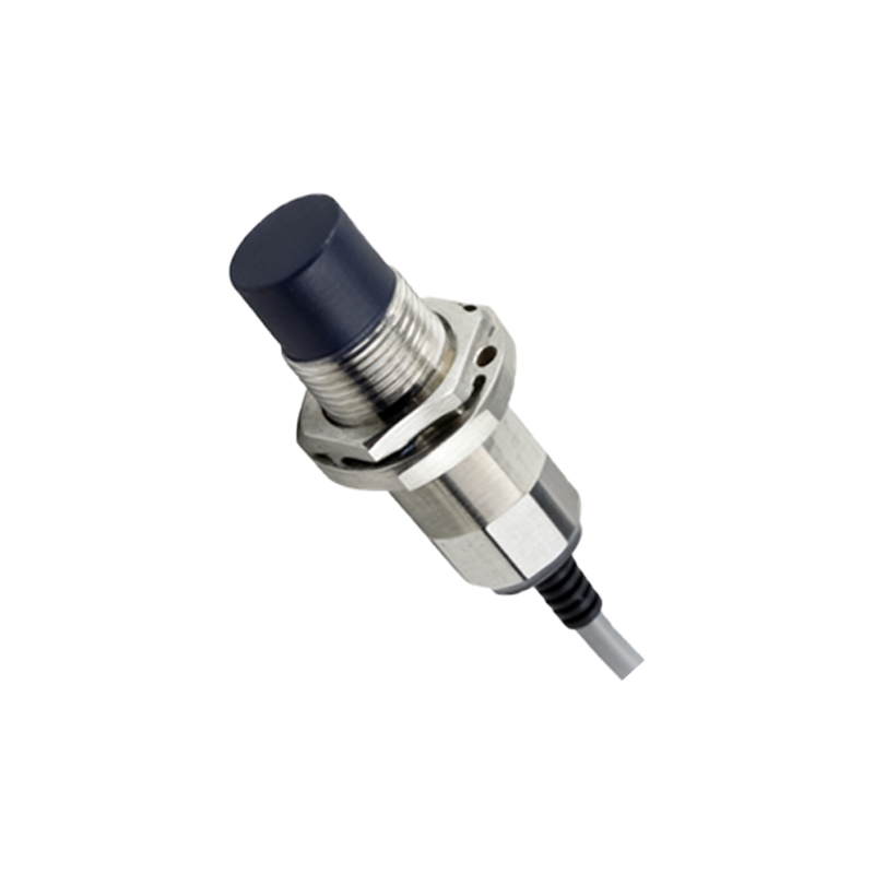
In practice, always consult the manufacturer's datasheet for specific curves, as they are based on empirical testing. Compare multiple curves if your application involves variable conditions—like mixed materials or temperature swings. Use the curves to calculate safety margins: for reliable operation, set the installation distance at 70-80% of the rated sensing distance to accommodate tolerances. Regularly validate performance during maintenance, as wear or contamination can alter sensing characteristics over time.
By mastering sensing curve analysis, engineers can optimize sensor selection, placement, and calibration, ensuring robust system performance. Whether deploying inductive, capacitive, ultrasonic, or photoelectric proximity sensors, these curves serve as a roadmap to precision and efficiency in automation.