Proximity sensors are ubiquitous in modern technology, silently enabling countless automated processes. At their core, these devices detect the presence or absence of an object within a specified range without physical contact. The underlying calculations that govern their operation are fundamental to their precision and reliability. This article delves into the computational principles behind the most common proximity sensor technologies.
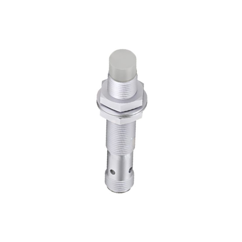
The operation of an inductive proximity sensor, primarily used for detecting metallic objects, relies on electromagnetic principles. The sensor generates an oscillating electromagnetic field. When a metallic target enters this field, eddy currents are induced on the target's surface. These currents draw energy from the sensor's oscillator circuit, causing a measurable change in its amplitude. The internal circuitry calculates this amplitude drop. The switching point, or the precise distance at which the sensor triggers an output signal, is determined by the sensor's design and the target material's properties, specifically its conductivity and permeability. For standard mild steel, a correction factor (often 1.0) is applied. For other metals like aluminum or copper, the effective sensing range (Sn) is calculated by multiplying the rated sensing distance by a material-specific factor (e.g., ~0.45 for aluminum). This ensures accurate detection regardless of the target material.
Capacitive sensors, capable of detecting both metallic and non-metallic objects, function by measuring changes in capacitance. The sensor face and the target act as two plates of a capacitor. The dielectric material (often air) between them completes the system. The capacitance (C) is proportional to the surface area of the plates (A), the dielectric constant of the material between them (ε), and inversely proportional to the distance (d) between the plates, as described by the formula C = εA/d. As a target approaches, the distance 'd' decreases or the effective dielectric constant changes, leading to an increase in capacitance. The sensor's electronics continuously calculate this capacitance value against a predefined threshold. Once the calculated value exceeds the threshold, the output state changes. This allows capacitive sensors to detect materials like plastic, wood, or liquids through thin container walls, with sensitivity adjustments compensating for different dielectric constants.
Ultrasonic sensors calculate distance using time-of-flight measurements. The sensor emits a high-frequency sound pulse and then listens for the echo. The core calculation is straightforward: Distance = (Speed of Sound × Time of Flight) / 2. The time of flight is the interval between pulse emission and echo reception. The speed of sound in air is approximately 343 meters per second at 20°C, but it varies with temperature, humidity, and air pressure. Advanced sensors incorporate temperature sensors to dynamically adjust the speed of sound constant in their distance calculation, significantly improving accuracy. The division by two accounts for the sound wave's round trip to the target and back. This calculation enables precise distance measurement, not just binary detection, making ultrasonic sensors ideal for level monitoring or positioning applications.
Photoelectric sensors, including through-beam, retro-reflective, and diffuse types, rely on light intensity calculations. In a diffuse (proximity) mode, the sensor emits a light beam (usually infrared or laser) and measures the intensity of the light reflected directly from the target. The received light intensity follows the inverse-square law, diminishing rapidly with increasing distance. The sensor's receiver converts light intensity into an electrical current. The internal circuit calculates whether this current signal strength exceeds a set threshold, which corresponds to the target being within the specified sensing window. Background suppression sensors perform more sophisticated calculations, using triangulation or time-of-flight principles to only respond to targets within a very specific, narrow range, ignoring objects farther away.
Beyond simple detection, calculations are crucial for handling real-world complexities. Hysteresis is a calculated dead band intentionally built into the sensor's logic. It prevents output chatter when a target is positioned at the exact switching point due to vibration or minor fluctuations. For instance, a sensor may switch on at 9mm and will not switch off again until the target moves beyond 11mm. This 2mm hysteresis is a calculated parameter ensuring stable operation.
Furthermore, modern smart sensors perform continuous self-diagnostics and calibration calculations. They monitor parameters like temperature drift, supply voltage stability, and signal-to-noise ratios, adjusting their internal thresholds dynamically to maintain optimal performance over time and in varying environmental conditions.
In application, understanding these calculations is key to proper sensor selection and installation. Engineers must consider the target size, material, required sensing distance, environmental factors (like dust or temperature), and the necessary response time. The calculations define the sensor's repeatability, linearity (for analog outputs), and overall system reliability. From assembly robots and packaging machinery to automotive safety systems and consumer electronics, the precise calculations performed by proximity sensors form the invisible logic that drives automation, ensuring efficiency, safety, and precision in a contactless world.