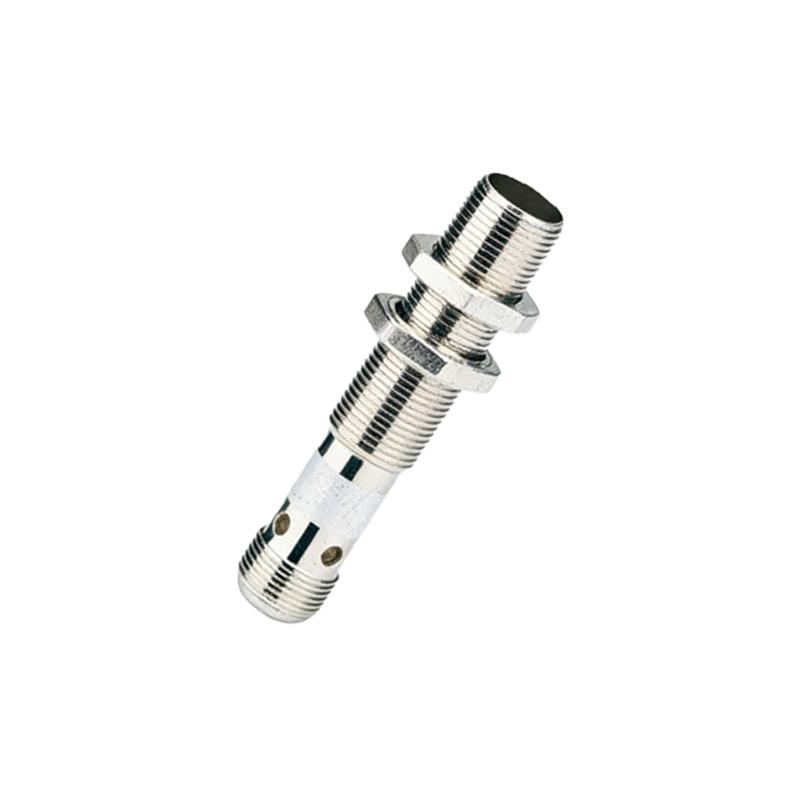
In the realm of industrial automation and electronic design, proximity sensors are indispensable components that detect the presence or absence of objects without physical contact. One critical aspect often scrutinized by engineers and designers is their power consumption, specifically the current draw, as it directly impacts system efficiency, battery life in portable applications, and overall operational costs. This article delves into the factors influencing the current consumption of proximity sensors, typical values across different types, and strategies for optimization.
Proximity sensors operate on various principles, including inductive, capacitive, ultrasonic, and optical (infrared) technologies. Each type exhibits distinct power characteristics. Inductive sensors, commonly used for metal detection, typically draw currents ranging from 10 mA to 30 mA in standard DC versions, with some low-power models consuming as little as 5 mA. Capacitive sensors, suited for non-metallic materials, often have similar current draws, averaging between 15 mA and 25 mA. Ultrasonic sensors, which emit sound waves, can be more power-hungry, with currents from 20 mA to 50 mA depending on the sensing range and frequency. Optical sensors, especially those with modulated infrared LEDs, may vary widely; basic models consume around 10 mA to 20 mA, while high-performance or long-range units can exceed 30 mA.
The current consumption is not constant and depends on several operational factors. Supply voltage plays a key role—most proximity sensors are designed for DC voltages like 12 V or 24 V, and higher voltages generally lead to slightly reduced current draw for the same power output due to Ohm's Law (P = VI). Sensing distance also affects power usage; longer ranges often require more energy to emit stronger signals, increasing current draw. Additionally, output configuration matters: sensors with transistor outputs (e.g., NPN or PNP) typically have lower quiescent currents (idle state) compared to those with relay or analog outputs, which may draw extra current during switching or signal transmission. Environmental conditions, such as temperature extremes, can cause fluctuations in current consumption due to changes in component efficiency.
In practice, engineers must consider both static and dynamic current. Static current refers to the baseline draw when the sensor is powered but not actively detecting, often in the range of 2 mA to 10 mA for modern low-power designs. Dynamic current spikes occur during object detection or output switching, potentially reaching 1.5 times the nominal value for brief periods. This is crucial for power supply sizing and avoiding voltage drops in sensitive circuits. For battery-operated devices, like in IoT or mobile robotics, minimizing average current is paramount. Techniques include using pulsed operation modes, where the sensor activates intermittently, reducing average draw to microampere levels, or selecting sensors with sleep or power-down features.
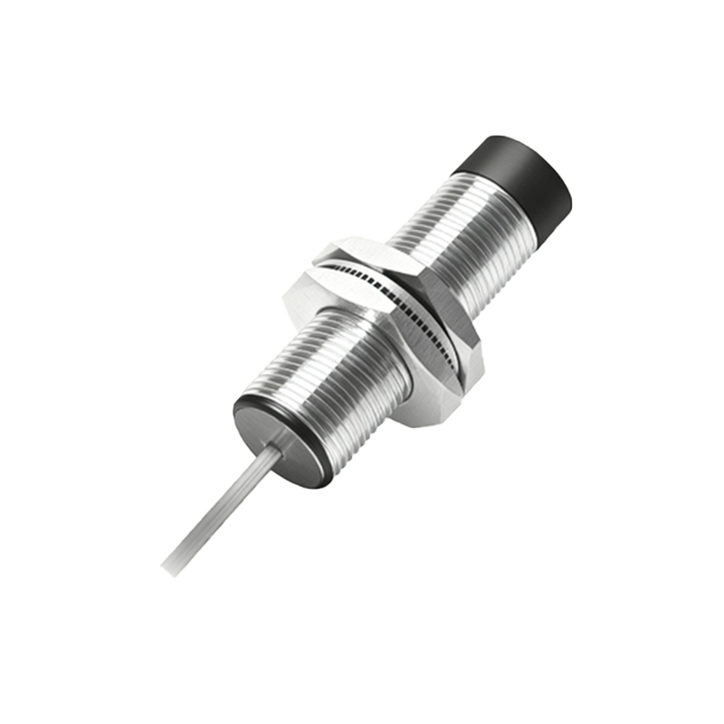
To optimize power consumption, start by selecting the right sensor type for the application. For instance, inductive sensors are efficient for metal detection in factory settings, while optical sensors might be better for low-power consumer electronics. Review datasheets carefully, focusing on parameters like "current consumption" or "supply current," often specified at nominal voltage and load. Implement power management circuits, such as MOSFET switches, to disable sensors when not in use. In wireless systems, consider energy-harvesting solutions to offset sensor power needs.
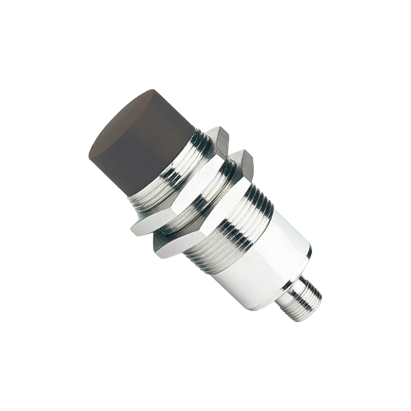
In summary, the current draw of proximity sensors is a multifaceted topic influenced by technology, design, and usage. By understanding these factors, engineers can make informed choices to balance performance with energy efficiency, ensuring reliable and sustainable operations across diverse industries from manufacturing to smart devices.